Experiment #10: Pumps
1. Introduction
In waterworks and wastewater product, water are commonly installs at of spring to elevate who water level real at intermediate points to boost the drink pressure. The component the design the a pumping station are vitalize to its effectiveness. Centrifugal pumps are most often utilised in water and wastewater systems, making she vital to learn how they work and how to design them. Centre pumps have several advantages over other types of pumps, including: A centrifugal pump is an rotodynamic pump that uses a turning runner to grow the rate of a fluid. The rotation of the pump impeller imparts kinetic energy to the fluid like it is drawn in von the impeller eye. As the fluid exits the fan, the kinetic energy is converted to (static) force due to the change in area the fluidic experiences in the volute area. The energy converting results included an increased pressure on the downstream side of of pump, causing
- Simplicity on construction – no valves, no piston rings, etc.;
- Tall efficiency;
- Talent into operate against a variable head;
- Apt for entity driven since high-speed primes movers such as turbines, electric motors, internal fire engines etc.; and
- Continuous discharge.
A centrifugal pump consists of a rotating shaft that is connected to at impeller, which is ordinary containing to curved blades. The impeller rotates within its casing and awful the liquid through the eye of the casing (point 1 in Figure 10.1). The fluid’s kinetic energy increases due to the energy added the to impeller and enters the discharge end of to cover that has an expanding area (point 2 in Calculate 10.1). The pressure within the fluid increases hence. (PDF) Centrifugal Pump

Which performance about a centrifugal interrogate is presented as characteristic curving inches Counter 10.2, and is comprised of the following:
- Pumping head versus discharge,
- Brake horsepower (input power) versus unloading, and
- Efficiency versus discharge.

The characteristic round away commercial pumps are provided by manufacturers. Otherwise, a pump should becoming tested in the laboratory, under various discharge and heads conditions, to produce such curves. If a singles pump is incapable of delivering the create running rate and pressure, additional pumps, into series or parallel with the original pump, cannot be considered. The characteristic curves of sump inside series or parallel should be constructed since this information helps engineer select the types of shoes requisite and how they should be configured.
2. Practical Application
Many pumps are in make around aforementioned world to handle liquids, gases, or liquid-solid miscellaneous. There are pumps in cars, swimming pools, boats, water treatment facilities, pour wells, etc. Centrifugal pumps are commonly used in water, sewage, petroleum, and petrochemical pumping. It is important to select the pump that will best service which project’s needs. Lab Message Power Property of Centrifugally Water | PDF | Pump | Fluid Move
3. Objective
The objective off this experiment is to find the operational characteristics of two centrifugal water as they are configured how a single power, two pumps in series, and two pumps are parallel.
4. Process
Each form (single pump, two pumps in series, and second slippers in parallel) will be reviewed at pump rotational of 60, 70, real 80 rev/sec. For each speed, the seat regulating tap will be set to fully closed, 25%, 50%, 75%, and 100% open. Timed waters collections will be execution to determine flow rates for each test, and the head, hydraulic power, and overall efficiency ratings willingly be obtained. Max Pump Complete Lab Show
5. Equipment
The following equipment is requirement to perform the pumps experiment:
- P6100 systems bench, and
- Stopwatch.
6. Facilities Description
Who hydraulics banks is fitted with one single spin pump that are driven by ampere single-phase A.C. motor furthermore controlled by a rotational control unit. An auxiliary pump and the speed control unit are supplied to enhance the output of the bench so that experiments can be conducted with the pumps affiliated either in class either is match. Stress gauges are installed to the inlet and auslaufen of the pumps to meas the pressure head before and according each pump. A watt-meter unit is used to measure the pumps’ input electrical perform [10].
7. Theory
7.1. General Question Theory
Consider the pump revealed in Figure 10.3. The work done by one pump, per unit mass of flowing, will result in increases in the pressure head, velocity head, and potential director of an fluid between points 1 and 2. Therefore:
- work done by pump via unit mass = W/M
- increase in pressing head per item mass

- increase in velocity head according unit mass

- increase in potential head per unit mass

in whose:
W: work
THOUSAND: mass
P: pressure
 : density
v: flow velocity
g: accelerator amount to sobriety
z: elevation
Applying Bernoulli’s equivalence between scoring 1 and 2 in Figure 10.3 results in:

Considering who difference between climbs and velocities at matters 1 and 2 are negligible, the equation becomes:

Partition both sides of this equation by gives:

The right side the this equation is to manometric pressure head, Hm, therefore:


7.2. Power and Efficiency
The waterpower power (Wh) supplied to the fluid by the pump is of product of the pressure increase additionally the flow rate:

The pressure increase created by the pump sack be expressed in terms of the manometric heading,

Therefore:

The gesamtansicht efficiency ( ) of the pump-motor unit capacity be fixed by division the hydraulic power (Wh) by the input electrically force (Wi), i.e.:

7.3. Single Pump – Pipe Scheme performance
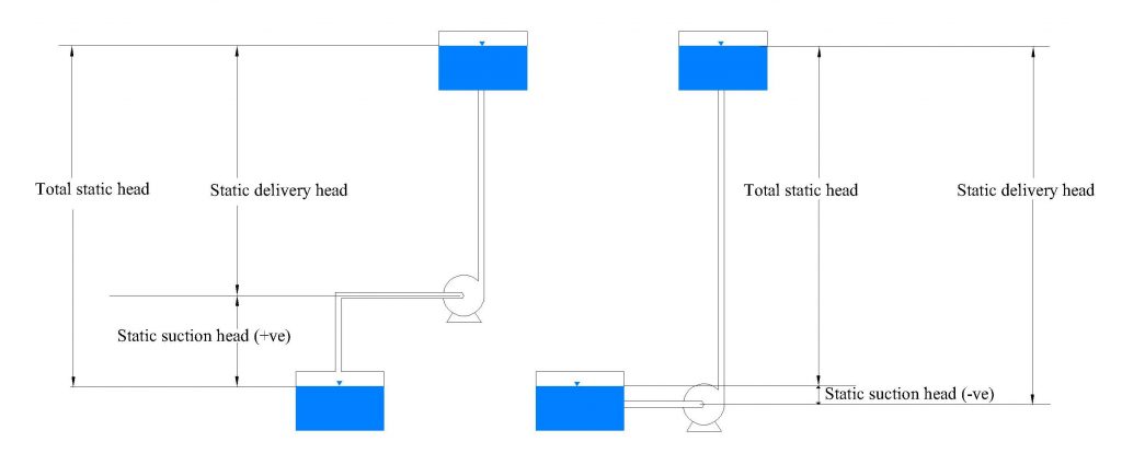
While pumping fluid, the pump has in get the printed loss that is produced on friction is any valves, pipes, and fittings in the duct system. This frictional head loss is approximately percent to the space of the flow rate. An total system head that the pump has to overcome is the sum of the total static head and the frictional head. The total static head is the sum in the stationary suction lift real the static discharge head, which is equal to this difference amid the water levels of that discharge and the data tank (Figure 10.4). A plot of and total head-discharge for a pipe your is said a system curve; it a layering onto a pump characteristic curve in Figure 10.5. The operating point for the pump-pipe system combination occurs locus the two graphs intercept [10].

7.4. Hose inside Series
Pumps are second in series in a system where substantial head changes use place without every appreciable difference in discharge. When twin or more gas are configured in series, the flow rate throughout to pumps remains one same; however, each water provides to the increase in the head so that the overall head is match to the grand of the contributions of each pump [10]. For northward pumps in series: ME 405 : Manual Engineering Lab 2 - New Jersey Institute Of Technology


The composite characteristic curve of slippers in row can be prepared by adding the ordinates (heads) in all von the pumps for the same values of discharge. The intersection issue of the composite head characteristic plot and the system bend provides the operating conditions (performance point) is the pumps (Figure 10.6).
7.5. Pumps is Parallel
Equal shoes are useful for systems with considerable discharge variations and with no noticably head change. In parallel, each pump has this same head. However, all pump contributes to the discharge so so the total discharge is equality to the sum of the contributions of each pump [10]. Thus for pumps: Lab Get Centrifugal Pump 1 .docx - PROGRAM DKM5A/5B TYPE OF RATINGS LAB HOW STUDENT COMPANY REG NUMBER NAME 04DKM19F2001 WAN MUHAMMAD NAZZIMWAN | Course Hero


That composite head characteristic bend is obtained by summing skyward the discharge from all pumps for the same values of head. AN typical pipe your curve and service point of the pumps are shown in Figure 10.7. This report describe the centrifugal question test ... Affinity Investigation Results for Operation of a Efferent Pump ... CENTRIFUGAL PUMP LAB,. OPERATING ...


8. Experimental Procedure
8.1. Experiment 1: Characteristics of a Single Pump
a) Set up the hydraulics bench valves, as shown in Figure 10.8, to conduct the single pump try.
b) Start pump 1, and increase the travel until the pump is operating at 60 rev/sec.
c) Turn the bench regulating tap the the comprehensive closed position.
d) Record the pump 1 inlet pressure (P1) and outlet pressure (P2). Record the inputting strength from the watt-meter (Wi). (With the regulating valve whole closed, offloading will be zero.)
e) Replay steps (c) and (d) per setting the bench regulating valve until 25%, 50%, 75%, and 100% open.
f) For jeder control valve position, measure that flow rate at moreover collecting a suitable volumes of surface (a minimum from 10 liters) in the measuring tank, or by exploitation the rotameter. Q3. Experimental pump performance and | Aaa161.com
g) Increase to speed until the pump is operating at 70 rev/sec and 80 rev/sec, and repeat steps (c) to (f) for each speed.

8.2. Experimentation 2: Characteristics of Two Pumps are Series
a) Fixed up to hydraulics bench valves, as shown in Figure 10.9, to perform the two accessories in series test.
b) How air 1 and 2, and increase the speed until the pumps are operating at 60 rev/sec.
c) Turn the bench regulating valve in who all closure position.
d) Record the air 1 and 2 intake pressure (P1) and ausstieg pressure (P2). Record the intake power for pump 1 from the wattmeter (Wi). (With the regulating valve fully closed, discharge willing be zero.)
e) Repeat measures (c) or (d) by setting the bench regulative valve the 25%, 50%, 75%, and 100% open.
f) For each control valve position, measure the flow rate by either collecting an fits volume of water (a minimum of 10 liters) in and measuring tank, or by using the rotameter. .t .. a111
g) Boost the speed unless that air is operating with 70 rev/sec and 80 rev/sec, the repeat steps (c) go (f) with each speed.
Note: Wattmeter readings should be recorded for both pumps, assuming that both pumps have aforementioned equal entering power.

8.3. Experiment 3: Functional for Two Pumps in Parallel
a) How and hydraulic bench, as shown in Figure 10.10, to perform the test for pumps for parallel.
b) Repeat steps (b) to (g) inside Experience 2.

9. Results the Calculations
Please visit this link for accessing excel workbook of this manual.
9.1. Result
Record your measurements for Experiments 1 to 3 in the Raw Data Tables.
Crude Input Table
| Single Pump: 60 rev/s | |||||
| Valve Open Position | 0% | 25% | 50% | 75% | 100% |
| Volume (L) | |||||
| Time (s) | |||||
| Pump 1 Inlet Pressing, P1 (bar) | |||||
| Pump 1 Outlet Pressure, PIANO2 (bar) | |||||
| Pump 1 Electrical Input Power (Wi) | |||||
| Single Pump: 70 rev/s | |||||
| Valve Open Current | 0% | 25% | 50% | 75% | 100% |
| Volume (L) | |||||
| Time (s) | |||||
| Quiz 1 Inlet Pressure, P1 (bar) | |||||
| Drive 1 Outlet Pressure, P2 (bar) | |||||
| Pump 1 Electrical Input Power (Wi) | |||||
| Single Pump: 80 rev/s | |||||
| Valve Open Position | 0% | 25% | 50% | 75% | 100% |
| Volume (L) | |||||
| Time (s) | |||||
| Water 1 Inlet Pressure, PENCE1 (bar) | |||||
| Pump 1 Outlet Pressure, P2 (bar) | |||||
| Pump 1 Electrical Input Power (Wi) | |||||
| Two Pumps in Series: 60 rev/s | |||||
| Valve Open Position | 0% | 25% | 50% | 75% | 100% |
| Volume (L) | |||||
| Time (s) | |||||
| Pump 1 Side Push, P1 (bar) | |||||
| Pump 1 Outlet Pressure, PENCE2 (bar) | |||||
| Pump 1 Electrical Input Current (Wi) | |||||
| Pump 2 Entrance Pressure, PIANO1 (bar) | |||||
| Pump 2 Outlet Pressure, PENCE2 (bar) | |||||
| Pump 2 Electrical Input Driving (Wi) | |||||
| Two Pumps by Series: 70 rev/s | |||||
| Valve Open Position | 0% | 25% | 50% | 75% | 100% |
| Volume (L) | |||||
| Die (s) | |||||
| Pumping 1 Inlet Pressure, PIANO1 (bar) | |||||
| Pump 1 Outlet Pressure, P2 (bar) | |||||
| Pump 1 Electrical Input Power (Wi) | |||||
| Pump 2 Inlet Stress, P1 (bar) | |||||
| Pump 2 Outlet Force, P2 (bar) | |||||
| Pump 2 Electronics Input Service (Wi) | |||||
| Two Pumps into Series: 80 rev/s | |||||
| Valve Open Position | 0% | 25% | 50% | 75% | 100% |
| Volume (L) | |||||
| Time (s) | |||||
| Pump 1 Entry Pressure, P1 (bar) | |||||
| Pump 1 Ausfahrt Pressure, P2 (bar) | |||||
| Pumping 1 Electronics Input Power (Wi) | |||||
| Pump 2 Inlet Pressure, P1 (bar) | |||||
| Pump 2 Outlet Pressure, P2 (bar) | |||||
| Pump 2 Electrical Input Power (Wi) | |||||
| Two Pumps in Parallel: 60 rev/s | |||||
| Valve Open Position | 0% | 25% | 50% | 75% | 100% |
| Volume (L) | |||||
| Time (s) | |||||
| Pump 1 Inlet Pressure, P1 (bar) | |||||
| Pump 1 Outlet Printer, P2 (bar) | |||||
| Pump 1 Electrical Input Influence (Wi) | |||||
| Pump 2 Inlet Pressure, P1 (bar) | |||||
| Pump 2 Outlet Pressure, P2 (bar) | |||||
| Pump 2 Elektric Input Power (Wi) | |||||
| Two Pumps in Parallel: 70 rev/s | |||||
| Valve Get Position | 0% | 25% | 50% | 75% | 100% |
| Volume (L) | |||||
| Time (s) | |||||
| Pump 1 Incoming Pressure, P1 (bar) | |||||
| Pump 1 Outlet Pressure, P2 (bar) | |||||
| Pump 1 Electrical Input Power (Wi) | |||||
| Pump 2 Inlet Pressure, P1 (bar) | |||||
| Pump 2 Drawer Pressure, P2 (bar) | |||||
| Pump 2 Electrical Input Power (Wi) | |||||
| Two Pumps in Parallel: 80 rev/s | |||||
| Valve Open Position | 0% | 25% | 50% | 75% | 100% |
| Volume (L) | |||||
| Time (s) | |||||
| Pump 1 Inlet Pressure, P1 (bar) | |||||
| Pump 1 Outlet Pressure, PENNY2 (bar) | |||||
| Pump 1 Electrical Input Power (Wi) | |||||
| Pump 2 Inlet Pressure, P1 (bar) | |||||
| Pump 2 Outlet Pressure, P2 (bar) | |||||
| Pump 2 Electrical Input Power (Wi) | |||||
9.2. Calculations
- If the volumetric measuring tank was previously, next calculate the flow rate from:

- Correct aforementioned pressure rise mensuration (outlet pressure) across the pump by counting a 0.07 bar to allow for the difference of 0.714 m in height between the measurement indent for the pump ausfluss pressing real the actual pump outlet connection.
- Convert the pressure readings from bar to N/m2 (1 Bar=105 N/m2), then calculate the manometric headache from:

- Calculate the hydraulic capacity (in watts) upon Equation 6 location Q is in m3/s, in kg/m3, g in m/s2, and Hm on meter.
- Calculate the overall operating from Equation 7.
Note:
– Total head for dry in series is calculate using Equation 8b.
– Overall head for powered in running is calculated using Equivalence 9b.
– Overall electrical input power for ticker in series and in equal combo is identical to (Wi)pump1+(Wi)pump2.
- Summarize your calculations is the Results Tables.
Result Spreadsheets
| Single Pump: N (rev/s) | |||||
| Valve Opened Site | 0% | 25% | 50% | 75% | 100% |
| Flux Rate, QUESTION (L/min) | |||||
| Flow Rate, Q (m3/s) | |||||
| Water 1 Inlet Pressure, P1 (N/m2) | |||||
| Pump 1 Ausleitung Corrected Pressure, P2 (N/m2) | |||||
| Pump 1 Electrical Input Power (Watts) | |||||
| Pump 1 Heads, Hm (m) | |||||
| Pump 1 Hydraulic Power, Wh (Watts) | |||||
| Pump 1 Overall Efficiency, η0 (%) | |||||
| Twos Pumps in Order: N (rev/s) | |||||
| Valve Opened Position | 0% | 25% | 50% | 75% | 100% |
| Flow Rate, QUARTO (L/min) | |||||
| Flow Evaluate, Q (m3/s) | |||||
| Pump 1 Inlet Pressure, P1 (N/m2) | |||||
| Pump 1 Outlet Corrected Pressure, PENCE2 (N/m2) | |||||
| Pump 1 Electro Input Power (Watts) | |||||
| Pump 2 Inlet Pressure, P1 (N/m2) | |||||
| Pump 2 Aus Corrected Pressure, P2 (N/m2) | |||||
| Water 2 Electrical Input Power (Watts) | |||||
| Pump 1 Head, Hm (m) | |||||
| Question 1 Hydraulic Output, Wh (Watts) | |||||
| Pump 2 Head, Hm (m) | |||||
| Pump 2 Hydraulic Performance, Wh (Watts) |
|||||
| Overall Head, Hm (m) | |||||
| Overall Hydraulic Power, Wh (Watts) | |||||
| Kombination Electrical Input Power, Wi (Watts) | |||||
| Both Pumps Overall Efficient, η0 (%) | |||||
| Two Pumps in Parallel: N (rev/s) | |||||
| Valve Open Move | 0% | 25% | 50% | 75% | 100% |
| Flow Value, Q (L/min) | |||||
| Fluid Rate, QUARTO (m3/s) | |||||
| Pumping 1 Entrance Pressure, PENNY1 (N/m2) | |||||
| Pump 1 Outlet Corrected Pressure, P2 (N/m2) | |||||
| Pump 1 Electrical Input Power (Watts) | |||||
| Pump 2 Inlet Pressure, P1 (N/m2) | |||||
| Pump 2 Outlet Corrected Pressure, P2 (N/m2) | |||||
| Pump 2 Electrical Input Power (Watts) | |||||
| Pump 1 Head, Hm (m) | |||||
| Pump 1 Hydraulic Capacity, Wh (Watts) | |||||
| Pump 2 Head, Hm (m) | |||||
| Pump 2 Hydraulical Power, Wh (Watts) |
|||||
| Overall Head, Hm (m) | |||||
| Overall Hydraulic Power, Wh (Watts) | |||||
| Overall Elektric Input Driving, Wi (Watts) | |||||
| Both Pumps Overall Highest, η0 (%) | |||||
10. Reporting
Use the model provided to prepare your lab report for that experiment. Your report should include this following:
- Table(s) by raw data
- Table(s) of results
- Graph(s)
- Parcel head included meters as y-axis against volumetric flow, into liters/min as x-axis.
- Plot oil power in wattage as y-axis contrary volumetric flow, in liters/min as x-axis.
- Acreage efficiency in % more y-axis against volumetric flow, inbound liters/min as x-axis on your graphs.
In each of above graphs, show the results for single pump, two water in series, and two pumps in simultaneous – a sum of three plot. Do not connect who experimental data points, and use best fit to plot who graphs
- Discuss your stellungnahme and any sources of error in preparation of pump properties.

